Learning Objectives
Use tools on the Galaxy platform to:
- Dig into a real metagenomics sample from the field.
- Import data and perform QC and quality filtering of your soil metagenome with the NanoPlot and fastp tools.
- Run taxonomy profiling workflow to classify and visualize taxonomy of a soil sample.
Throughout this activity you will also compare soil and gut metagenomes.
Introduction
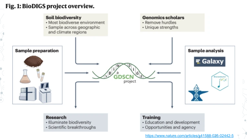
The BioDIGS (BioDiversity and Informatics for Genomics Scholars) Project is a nationwide initiative involving students, researchers, and educators across more than 40 research and teaching institutions. Participants collect samples, analyze data, and interpret results to understand the relationships between the soil microbiome, environment, and health.
Note, the total time for a Galaxy step to complete depends on and will increase based on multiple factors such as the input file size, a long queue when many other people are analyzing data, the complexity of the job itself and errors. See the table below for the minimum time a step will take for this assignment – be sure to start early as when Galaxy is busy each step can take 2-to-10 times longer to complete.
Table of approximate minimum times for a job to be completed on Galaxy using specified tools.
| 10 min |
10 min |
15 min |
30 min |
Note, you can save time by:
- Submitting multiple jobs that use the same input (NanoPlot and fastp)
- Submitting a job like the taxonomy workflow that uses the fastp output as input as soon as the output appears in your history even before the fastp job is complete.
Activity 1 – Data import and QC
Estimated time: 50 min
Part 1 - Import data and run NanoPlot
Instructions
- Import the dataset into Galaxy.
- Open the nanopore soil subset from a public history BioDIGS_PromethION-M01_1_subset
- Click on
Import this history, select Copy only the active, non-deleted datasets and then Copy History.
- Confirm BioDIGS_PromethION-MO1_1_subset exists in your history by clicking on the Home button on top left.
- Run the NanoPlot tool in Galaxy to assess sequence quality using the default settings.
- Click on the Tools icon. Then, in the search bar enter ‘NanoPlot’ and select the NanoPlot tool.
- Under files browse to select your BioDIGS_PromethION-MO1_1_subset fastq dataset.
- Click on Run Tool and wait ~10 minutes as the NanoPlot job is scheduled, run, and completed.
Questions
| Read mean length (mean read length): |
|
| Read Mean quality (mean_qual): |
|
| Proportion of reads with quality > Q20 (Reads > Q20): |
|
- Compare soil NanoPlot results with the gut NanoPlot results.
| mean read length: |
|
|
| mean_qual: |
|
|
| Reads with > Q10 bases (%): |
|
|
Part 2 - Quality filtering with fastp
Instructions
Filtering raw sequencing reads is a common step to improve data quality before downstream analysis. Nanopore datasets often include reads with relatively low base-call quality - for example, bases below a Phred quality score of Q10 - which should match what you observed in your NanoPlot results above.
Given this, we will apply a stricter quality filter using a Phred threshold of Q20. This means that we will retain only reads that on average meet the chosen Q20 criterion, and discard lower-quality reads to improve the reliability of subsequent analysis.
NOTE: Unlike Nanopore reads, PacBio HiFi (High Fidelity) reads are already at Q20 or above, so quality filtering of PacBio HiFi is typically not required.
- Run fastp tool to filter out reads with an average quality score of less than Q20. In fastp, the default filtering is based on Phred quality score of 15 (Q15). To filter based on Phred quality score of 20 (Q20) adjust tool parameters:
- Click on the Tools icon. Then, in the search bar enter fastp and select the fastp tool.
- Under Filter Options, in an empty Qualified quality phred box, enter 20 (indicating Q20).
- Click on Run Tool and wait ~10-15 minutes as the fastp job is scheduled, run, and completed.
Questions
- Compare your dataset BEFORE and AFTER filtering using fastp: HTML report output.
| Mean Length |
|
|
| total reads |
|
|
| Q20 bases (%): |
|
|
Activity 2 – Taxonomy Profiling
Estimated time: 50 min (~35 min computing)
Part 1 - Run Taxonomy Profiling Workflow
Instructions
- Run the ‘Taxonomy Profiling’ workflow on your fastp-filtered data from Activity 1 and view the results.
- Open the taxonomy-profiling public workflow https://usegalaxy.org/u/cutsort/w/taxonomy-profiling.
- Click on Run.
- Browse to select your fastp-filtered fastq dataset “fastp on data1:Read 1 output” dataset by clicking on the
‘...’ tab.
- Under kraken_database select Prebuilt Refseq indexes: PlusPF(Standard plus protozoa and fungi)(Version:2022-06-07 - Downloaded: 2022-09-04T165121Z).
- Click Run Workflow.
- Wait ~30 minutes as the Kraken 2, KrakenTools, and Krona jobs are scheduled, run, and completed.
- Click on the Display icon (eyeball) next to the output file with converted_kraken_report. Explore the metagenomic diversity of the soil sample by performing the taxonomy profiling spreadsheet activity you did during week 1.
- Click on converted_kraken_report, find the download button and download the report.
- Change the extension of your taxonomy file from .tabular to .tsv.
- Upload your taxonomy .tsv file to Google Drive and open it with Google Sheets.
- Create a header row and enter the following column information.
- Col A = Counts.
- Cols B-H correspond to taxonomic ranks k(Kingdom), p(Phylum), c(Class), o(Order), f(Family), g(Genus) and s(Species).
- Each row corresponds to a different taxa.
- Evaluate what proportion of data was taxonomically classified.
- Insert a new column A; we will use this temporary column for calculations, so you can name this column “Calculations”.
- In e.g. cell A2, calculate the sum of all reads observed in the soil sample.
Questions
- Identify the most abundant taxa (those at >0.1%).
- Remember, soil is one of the most diverse microbial environments with many more microbial species than in the gut. Therefore, abundant species can still be quite low abundance.
- Select columns B through I.
- In the Data menu, select “Sort range by column B (Z to A)”.
- Insert a new column C.
- we will use this temporary column for calculations;
- you can name this column “% abundance”.
- In new column C, calculate % abundance for each row.
- by dividing each count value by the total number of reads and multiplying by 100.
Part 2 - Analyze Kraken 2 results
Instructions
- Click on the Display icon (eyeball) next to the output file with kraken2_with_pluspf_database_output_report. This output report is an extended version of the converted_kraken_report. The output contains 6 columns. See info for select column headers below:
- Column 1: Percentage (%) of a given taxon
- Column 2: # of reads per given taxon
- Column 4: A rank code, indicating (U)nclassified, (R)oot, (D)omain, (K)ingdom, (P)hylum, (C)lass, (O)rder, (F)amily, (G)enus, or (S)pecies. Note, that in this extended file, some rank codes will have numbers associated with them; Ignore this aspect of the document for the moment.
- Column 6: Identified taxa/scientific name.
- Of note: The benefit of kraken2_with_pluspf_database_output_report is that it summarizes converted_kraken_report and calculates summary percentages for taxonomic ranks. For example, your converted_kraken_report has hundreds of lines for phylum Proteobacteria, while kraken2_with_pluspf_database_output_report has 1 line summarizing the percent abundance of all Proteobacteria.
Instructions
Krona pie chart is one of the outputs of the taxonomy workflow, and it is an interactive visualization tool for exploring the composition of metagenomes.
- View the Krona results: Click on the Display icon (eyeball) next to the output file named krona_pie_chart.
- Double click on Bacteria kingdom (k_Bacteria) to explore further.
- Answer questions below
Questions
- Use Krona and/or Kraken2 outputs to compare your taxonomy from this soil sample, to the gut taxonomy results from your taxonomy-prelab (Zymo-gut-standard ZymoBIOMICS® Gut Microbiome Standard
3A. Fill out the comparison table below
| What are 2 most abundant phyla |
|
|
| What are 2 most abundant species |
|
|
| % Classified taxa |
|
|
| % Unclassified taxa |
|
|
|
|
|